hexagon logo

Ideas for smoothing solid-flex contacts (PSHELL)?

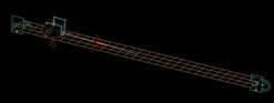
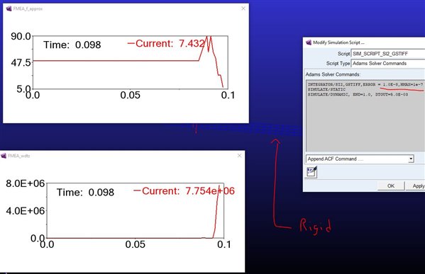
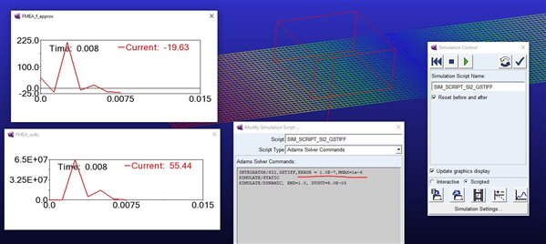
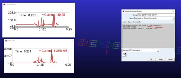
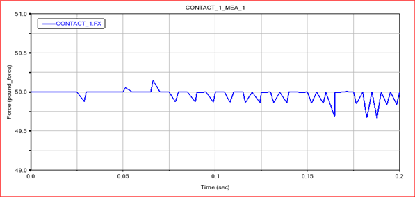
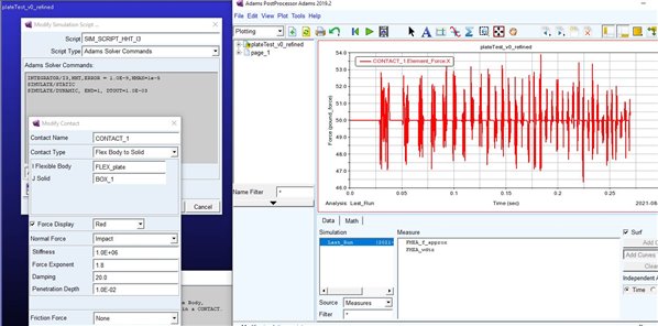
Attached model drags a simple block across a simple flexible plate's surface. Force is too unsteady to be of any use. Even with flexbody rigid, force is unsteady.
 
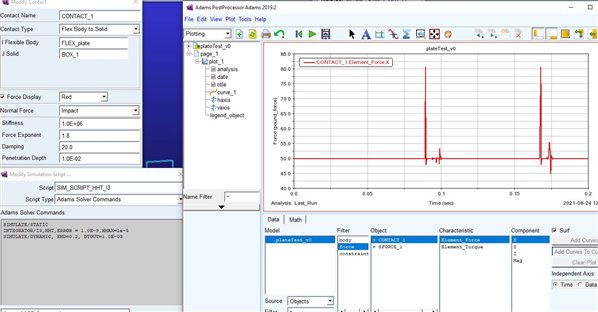
I've noticed using SI2 solver dramatically helps, but hoping someone out there has other tricks up their sleeve (other than just softening the contact parameters).

Attached Files (2)
  • Hi Erik,
     
    With any computational tool, you would need to perform a convergence study (integrator sensitivity analysis) to make sure that the results are not dependent on the integrator settings (e.g., ERROR and HMAX). In such attempt, you need to tighten ERROR and HMAX and find a contact force that is not dependent on these parameters. Only then, will the results be reliable.
     
    Now, since this is a contact model, you would need refrain from using GSTIFF/I3 integrator. GSTIFF/SI2 and HHT/I3 are to be your choices. With both you would need to perform a convergence study. The HHT integrator is, however, more sensitive to HMAX values.
     
    Thank you,
    Maziar Rostamian
    MSC Software
     
    Thank you,
    Maziar
  • I also strongly recommend that you review WM466 webinar on SimCompanion.
  • Thanks. I definitely did appear to take these valid and important considerations for granted. Indeed, reducing error and hmax does resolve.
     
    But the intent of my question was a bit different. More or less, what you're suggesting is a brute force approach that results in a smaller timesteps / longer run times. I was hoping to get some feedback on alternative approaches that inherently result in more stable solutions, shorter run times.
     
    For example, splitting the block into 3 spheres appears to improve performance (attached "v1")
     
    In attached "v2", noting that even the rigidized mesh had convergence issues, I created an identical grid of blocks merged to ground, which resulted in better (but not perfect) behavior. I guess understanding why this would work better than the original mesh is at the heart of the question.
     
    If I had to guess, it appears as if the number of contact traces tends to vary a lot, changing the effective center-of-contact, and resulting in poor behavior (at large error/hmax). This would be why the "v1" sphere approach acts better, since spheres always result in 3 traces at fixed locations.
     
    But, in all this, I guess I don't really have another question. bit please comment if this spurs some related thoughts.

    Attached Files (1)
  • The sensitivity analysis is more of a crucial step than a brute force approach that needs to be done regardless of how you model your mechanism.
     
    Splitting the geometry into multiple geometries has two advantages:
     
    1. The contact detection algorithm will not have to deal with large geometries throughout the whole simulation. In other words, when you have multiple geometries in multiple contact objects instead of one large geometry in one contact object, the contact detection algorithm will only be working on one of these geometries at a time and can therefore, return contact node pairs faster.
    2. In this case, you can take advantage of multi-threading better, in that, the solver can split these contact objects among the available threads.
     
    Your examples V1 and V2 are totally different models, in that, the spheres contact with the flexible body occurs on almost on a line while the box contact with the flexible body occurs on a much wider surface. Moreover, the spheres come into a smooth contact with the flexible body due to the surface curvature while the box comes into sharp contact at its corners.
     
    Please also note that the the mesh refinement on the flexible body directly affects the contact results by affecting contact force symmetry and smoothness of the resolved contact force.
     
    Thank you,
    Maziar
  • Can you help me figure out how to get it to converge (better)?
     
    The model is a pretty simple illustration of sliding of a solid on a flex body surface, sharp corners or not. Seems like it'd be useful for anyone encountering the same issue in the future.
     
    The three pictures show the original coarse mesh and another model with a refined mesh, per your feedback. As seen, I've tried ERROR=1e-7, HMAX=1e-6, still not converging. On a rigidized mesh, I used ERROR=1E-8 and HMAX=1e-7 and didn't converge. (Plot shows large deviation from the 50 lbf contact load and large variance in angular acceleration about Z). It does run quite well for a short time, but then large blips in angular acceleration start to show up.
     
    These run times were well beyond expectation for the apparent simplicity of the models, borderline unusable but for sake of solving the problem, which is where the attribution to 'brute force' approaches came to mind--sorry about the use of the term "brute force", again, not to dismiss the need for care in this area, for such problems in general.
     
    Currently, the models I'm applying this generic concept to do use the v1 sphere approximation. Actual geometry, with sharp edges and all, would be preferred, though. My next thought would be to split the box in sub-sections, then apply to the refined mesh version (several grid elements per box segment). So, it'll end up being much like the spheres, but with shapes that better represent true geometry.
     
    Rigid_not_converging
     
    Refined_not_converging
    Original_not_converging

    Attached Files (1)
  • In your approach you have a sim/sta statement and you try to change ERROR & HMAX in order to improve "convergence".
    Unfortunately it's as helpful as filling up your wiper reservoir when the dashboard shows low engine oil.
    (Both parameters only influence dynamic solution, but the "convergence" message is from the static solver)
     
    In a nutshell: Static and dynamic solver are two different things.
    By sim/sta you order ADAMS to first find a static solution which is always VERY tricky with contacts. Almost none of my models find equilibrium when contacts are active.
    My usual approach is to skip the sim/sta command and let an initial dynamic phase with very small tome steps do the "equillibrium".
    The other method would be first to use "very small steps for static solution" by limiting TLIM/ALIM to small values and increase MAXIT.
    An additional trick is to stage multiple static commands one after another ("funneling") until an equilibrium could be found. Something like:
    EQUILIBRIUM/tlim=1,alim=1,maxit=100
    ! Funneling fuer Statik
    EQUILIBRIUM/error=10,stability=5,imbalance=10
    sim/stat
    EQUILIBRIUM/error=1,stability=1,imbalance=1
    sim/stat
    EQUILIBRIUM/error=0.1,stability=0.1,imbalance=0.1
    sim/stat
    EQUILIBRIUM/error=0.01,stability=0.01,imbalance=0.01
    sim/stat
    ! Start the dynamic analysis
    Activate/MOTION,ID= 3
    simulate/dynamics, END=3.0, dtout=5E-03
     
     
  • The settings are indeed for the dynamic solver, it just starts with a static solution, which was not showing any obvious shortcomings.
     
    If you have time/motivation, can you please run the simulation with the attached files as requested some time today?
     
    Again, the goal would be a smooth contact force (50 lbf) from t=0 to t=1. I don't care if the plate is flexible, or made rigid. Really just care about getting smooth contact forces with the flex body's surface.
     
    Instead, even at very low Error & Hmax, we see huge variation in angular acceleration about z-axis, after some time has passed.
  • You would still need to investigate the equilibrium settings to make sure that the system has achieved proper equilibrium prior to the dynamic simulation.
     
    However, the main issue here is the contact parameters. I see that you have worked on your integrator settings to minimize the effect of integrator ERROR and HMAX on the results, which is great, but you do need to investigate the contact parameters thoroughly. A very helpful resource would be  WM466 SimAcademy webinar on SimCompanion website, as I had noted earlier.
     
    I did not spend much time on the model but with the following contact parameters:
     
    K=1E6, e=1.8, Cmax=20, dmax=0.01
     
    and the following integrator settings:
     
    INTEGRATOR/HHT,I3,ERR=1.0E-9,HMAX=1E-5
     
    you will be able to achieve very good contact normal force time history:
     
    contact_force
     
    Thank you,
    Maziar
  • Thanks for your responses.
     
    Didn't see quite the same,
    • From "v0" (1st picture), was not matching
    • From "v0_refined", it was similar, but not quite as good (2nd picture).--this was with the flexbody set to rigid.
    Using 2019.2--probably older than yours--all other solver settings should be default.
     
    Anyway, fine at leaving it at this. Takeaways for me are that sliding contact, even for VERY SIMPLE models, requires significant changes to solver settings (10e6 lower-than-default ERROR, etc). Shouldn't be surprised if the converged ERROR/HMAX results in long run times, also shouldn't expect any Hertzian-based contact parameters to work well, as biasing towards lower stiffness will significantly assist convergence. If other approaches (such as using spheres) are applicable, then that's an obvious route to go, as long as the tradeoff with geometric accuracy is acceptable, weighted against run time.
     
    ver2019.2
    ver2019.2_ref2
     
  • Hi Erik,
     
    This was a good summary of takeaways from this thread, which I am sure will be helpful to other readers as well. I need to address a couple of points through:
     
    The simplicity of the model is not defined by the geometries or the number of DOFs necessarily. In some cases, a model with simple geometries and a limited number of DOFs can be deemed complex if it involves a nonlinear object such as contact and a flexible body used in contact, which makes the mesh refinement an extra deciding factor apart from the modal content of it. Moreover, if the accelerations terms are used to define the accuracy of the model, then such criteria for model validation can make the whole model verification and validation COMPLEX.
     
    The Hertzian contact approximation can be used as a ballpark to start an iterative process to find the actual contact parameters in a dynamic system.
     
    Thank you,
    Maziar